使用Transformer模型进行时间序列预测实战

时间序列预测是一个经久不衰的主题，受自然语言处理领域的成功启发，transformer模型也在时间序列预测有了很大的发展。本文可以作为学习使用Transformer 模型的时间序列预测的一个起点。

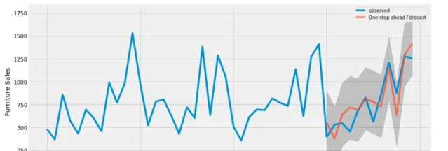
这里我们直接使用kaggle中的 Store Sales — Time Series Forecasting作为数据。这个比赛需要预测54家商店中各种产品系列未来16天的销售情况，总共创建1782个时间序列。数据从2013年1月1日至2017年8月15日，目标是预测接下来16天的销售情况。虽然为了简洁起见，我们做了简化处理，作为模型的输入包含20列中的3,029,400条数据，。每行的关键列为' store_nbr '、' family '和' date '。数据分为三类变量:

1、截止到最后一次训练数据日期(2017年8月15日)之前已知的与时间相关的变量。这些变量包括数字变量，如「销售额」，表示某一产品系列在某家商店的销售额;「transactions」，一家商店的交易总数;' store_sales '，该商店的总销售额;' family_sales '表示该产品系列的总销售额。

2、训练截止日期(2017年8月31日)之前已知，包括「onpromotion」(产品系列中促销产品的数量)和「dcoilwtico」等变量。这些数字列由' holiday '列补充，它表示假日或事件的存在，并被分类编码为整数。此外，' time_idx '、' week_day '、' month_day '、' month '和' year '列提供时间上下文，也编码为整数。虽然我们的模型是只有编码器的，但已经添加了16天移动值「onpromotion」和「dcoilwtico」，以便在没有解码器的情况下包含未来的信息。

3、静态协变量随着时间的推移保持不变，包括诸如「store_nbr」、「family」等标识符，以及「city」、「state」、「type」和「cluster」等分类变量(详细说明了商店的特征)，所有这些变量都是整数编码的。

我们最后生成的df名为' data_all '，结构如下:

 categorical_covariates = ['time_idx','week_day','month_day','month','year','holiday']
 categorical_covariates_num_embeddings = []
for col in categorical_covariates:
data_all[col] = data_all[col].astype('category').cat.codes
categorical_covariates_num_embeddings.append(data_all[col].nunique())
 categorical_static = ['store_nbr','city','state','type','cluster','family_int']
 categorical_static_num_embeddings = []
for col in categorical_static:
data_all[col] = data_all[col].astype('category').cat.codes
categorical_static_num_embeddings.append(data_all[col].nunique())
 numeric_covariates = ['sales','dcoilwtico','dcoilwtico_future','onpromotion','onpromotion_future','store_sales','transactions','family_sales']
 target_idx = np.where(np.array(numeric_covariates)=='sales')[0][0]





在将数据转换为适合我的PyTorch模型的张量之前，需要将其分为训练集和验证集。窗口大小是一个重要的超参数，表示每个训练样本的序列长度。此外，' num_val '表示使用的验证折数，在此上下文中设置为2。将2013年1月1日至2017年6月28日的观测数据指定为训练数据集，以2017年6月29日至2017年7月14日和2017年7月15日至2017年7月30日作为验证区间。

同时还进行了数据的缩放，完整代码如下：

defdataframe_to_tensor(series,numeric_covariates,categorical_covariates,categorical_static,target_idx):
numeric_cov_arr = np.array(series[numeric_covariates].values.tolist())
category_cov_arr = np.array(series[categorical_covariates].values.tolist())
static_cov_arr = np.array(series[categorical_static].values.tolist())
x_numeric = torch.tensor(numeric_cov_arr,dtype=torch.float32).transpose(2,1)
x_numeric = torch.log(x_numeric+1e-5)
x_category = torch.tensor(category_cov_arr,dtype=torch.long).transpose(2,1)
x_static = torch.tensor(static_cov_arr,dtype=torch.long)
y = torch.tensor(numeric_cov_arr[:,target_idx,:],dtype=torch.float32)
return x_numeric, x_category, x_static, y

 window_size = 16
 forecast_length = 16
 num_val = 2
 val_max_date = '2017-08-15'
 train_max_date = str((pd.to_datetime(val_max_date) - pd.Timedelta(days=window_size*num_val+forecast_length)).date())
 train_final = data_all[data_all['date']<=train_max_date]
 val_final = data_all[(data_all['date']>train_max_date)&(data_all['date']<=val_max_date)]
 train_series = train_final.groupby(categorical_static+['family']).agg(list).reset_index()
 val_series = val_final.groupby(categorical_static+['family']).agg(list).reset_index()
 x_numeric_train_tensor, x_category_train_tensor, x_static_train_tensor, y_train_tensor = dataframe_to_tensor(train_series,numeric_covariates,categorical_covariates,categorical_static,target_idx)
 x_numeric_val_tensor, x_category_val_tensor, x_static_val_tensor, y_val_tensor = dataframe_to_tensor(val_series,numeric_covariates,categorical_covariates,categorical_static,target_idx)









数据加载器

在数据加载时，需要将每个时间序列从窗口范围内的随机索引开始划分为时间块，以确保模型暴露于不同的序列段。

为了减少偏差还引入了一个额外的超参数设置，它不是随机打乱数据，而是根据块的开始时间对数据集进行排序。然后数据被分成五部分——反映了我们五年的数据集——每一部分都是内部打乱的，这样最后一批数据将包括去年的观察结果，但还是随机的。模型的最终梯度更新受到最近一年的影响，理论上可以改善最近时期的预测。

defdivide_shuffle(df,div_num):
space = df.shape[0]//div_num
division = np.arange(0,df.shape[0],space)
return pd.concat([df.iloc[division[i]:division[i]+space,:].sample(frac=1) for i in range(len(division))])
defcreate_time_blocks(time_length,window_size):
start_idx = np.random.randint(0,window_size-1)
end_idx = time_length-window_size-16-1
time_indices = np.arange(start_idx,end_idx+1,window_size)[:-1]
time_indices = np.append(time_indices,end_idx)
return time_indices
defdata_loader(x_numeric_tensor, x_category_tensor, x_static_tensor, y_tensor, batch_size, time_shuffle):
num_series = x_numeric_tensor.shape[0]
time_length = x_numeric_tensor.shape[1]
index_pd = pd.DataFrame({'serie_idx':range(num_series)})
index_pd['time_idx'] = [create_time_blocks(time_length,window_size) for n in range(index_pd.shape[0])]
if time_shuffle:
index_pd = index_pd.explode('time_idx')
index_pd = index_pd.sample(frac=1)
else:
index_pd = index_pd.explode('time_idx').sort_values('time_idx')
index_pd = divide_shuffle(index_pd,5)
indices = np.array(index_pd).astype(int)
for batch_idx in np.arange(0,indices.shape[0],batch_size):
cur_indices = indices[batch_idx:batch_idx+batch_size,:]
x_numeric = torch.stack([x_numeric_tensor[n[0],n[1]:n[1]+window_size,:] for n in cur_indices])
x_category = torch.stack([x_category_tensor[n[0],n[1]:n[1]+window_size,:] for n in cur_indices])
x_static = torch.stack([x_static_tensor[n[0],:] for n in cur_indices])
y = torch.stack([y_tensor[n[0],n[1]+window_size:n[1]+window_size+forecast_length] for n in cur_indices])
yield x_numeric.to(device), x_category.to(device), x_static.to(device), y.to(device)
defval_loader(x_numeric_tensor, x_category_tensor, x_static_tensor, y_tensor, batch_size, num_val):
num_time_series = x_numeric_tensor.shape[0]
for i in range(num_val):
for batch_idx in np.arange(0,num_time_series,batch_size):
x_numeric = x_numeric_tensor[batch_idx:batch_idx+batch_size,window_size*i:window_size*(i+1),:]
x_category = x_category_tensor[batch_idx:batch_idx+batch_size,window_size*i:window_size*(i+1),:]
x_static = x_static_tensor[batch_idx:batch_idx+batch_size]
y_val = y_tensor[batch_idx:batch_idx+batch_size,window_size*(i+1):window_size*(i+1)+forecast_length]
yield x_numeric.to(device), x_category.to(device), x_static.to(device), y_val.to(device)













模型

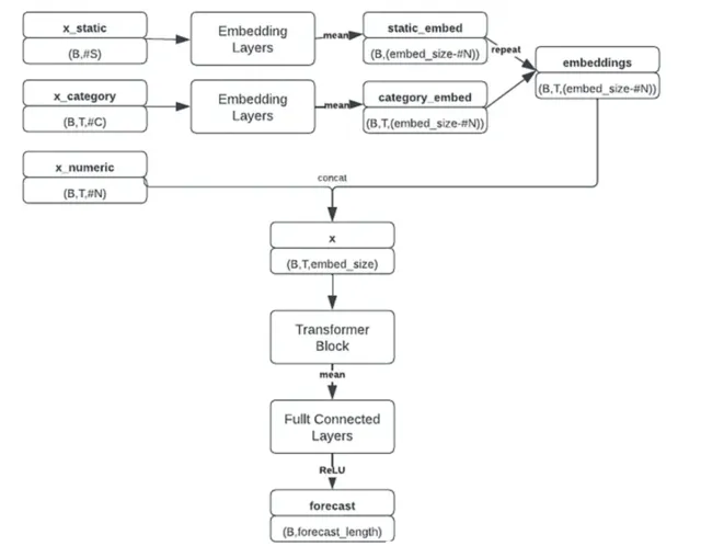
我们这里通过Pytorch来简单的实现【Attention is All You Need】(2017)²中描述的Transformer架构。因为是时间序列预测，所以注意力机制中不需要因果关系，也就是没有对注意块应用进行遮蔽。

从输入开始:分类特征通过嵌入层传递，以密集的形式表示它们，然后送到Transformer块。多层感知器(MLP)接受最终编码输入来产生预测。嵌入维数、每个Transformer块中的注意头数和dropout概率是模型的主要超参数。堆叠多个Transformer块由' num_blocks '超参数控制。

下面是单个Transformer块的实现和整体预测模型:

classtransformer_block(nn.Module):
def__init__(self,embed_size,num_heads):
super(transformer_block, self).__init__()
self.attention = nn.MultiheadAttention(embed_size, num_heads, batch_first=True)
self.fc = nn.Sequential(nn.Linear(embed_size, 4 * embed_size),
nn.LeakyReLU(),
nn.Linear(4 * embed_size, embed_size))
self.dropout = nn.Dropout(drop_prob)
self.ln1 = nn.LayerNorm(embed_size, eps=1e-6)
self.ln2 = nn.LayerNorm(embed_size, eps=1e-6)
defforward(self, x):
attn_out, _ = self.attention(x, x, x, need_weights=False)
x = x + self.dropout(attn_out)
x = self.ln1(x)
fc_out = self.fc(x)
x = x + self.dropout(fc_out)
x = self.ln2(x)
return x
classtransformer_forecaster(nn.Module):
def__init__(self,embed_size,num_heads,num_blocks):
super(transformer_forecaster, self).__init__()
num_len = len(numeric_covariates)
self.embedding_cov = nn.ModuleList([nn.Embedding(n,embed_size-num_len) for n in categorical_covariates_num_embeddings])
self.embedding_static = nn.ModuleList([nn.Embedding(n,embed_size-num_len) for n in categorical_static_num_embeddings])
self.blocks = nn.ModuleList([transformer_block(embed_size,num_heads) for n in range(num_blocks)])
self.forecast_head = nn.Sequential(nn.Linear(embed_size, embed_size*2),
nn.LeakyReLU(),
nn.Dropout(drop_prob),
nn.Linear(embed_size*2, embed_size*4),
nn.LeakyReLU(),
nn.Linear(embed_size*4, forecast_length),
nn.ReLU())
defforward(self, x_numeric, x_category, x_static):
tmp_list = []
for i,embed_layer in enumerate(self.embedding_static):
tmp_list.append(embed_layer(x_static[:,i]))
categroical_static_embeddings = torch.stack(tmp_list).mean(dim=0).unsqueeze(1)
tmp_list = []
for i,embed_layer in enumerate(self.embedding_cov):
tmp_list.append(embed_layer(x_category[:,:,i]))
categroical_covariates_embeddings = torch.stack(tmp_list).mean(dim=0)
T = categroical_covariates_embeddings.shape[1]
embed_out = (categroical_covariates_embeddings + categroical_static_embeddings.repeat(1,T,1))/2
x = torch.concat((x_numeric,embed_out),dim=-1)
for block in self.blocks:
x = block(x)
x = x.mean(dim=1)
x = self.forecast_head(x)
return x



















我们修改后的transformer架构如下图所示：

模型接受三个独立的输入张量:数值特征、分类特征和静态特征。对分类和静态特征嵌入进行平均，并与数字特征组合形成具有形状(batch_size, window_size, embedding_size)的张量，为Transformer块做好准备。这个复合张量还包含嵌入的时间变量，提供必要的位置信息。

Transformer块提取顺序信息，然后将结果张量沿着时间维度聚合，将其传递到MLP中以生成最终预测(batch_size, forecast_length)。这个比赛采用均方根对数误差(RMSLE)作为评价指标，公式为:

鉴于预测经过对数转换，预测低于-1的负销售额(这会导致未定义的错误)需要进行处理，所以为了避免负的销售预测和由此产生的NaN损失值，在MLP层以后增加了一层ReLU激活确保非负预测。

class RMSLELoss(nn.Module):
def __init__(self):
super().__init__()
self.mse = nn.MSELoss()
def forward(self, pred, actual):
return torch.sqrt(self.mse(torch.log(pred + 1), torch.log(actual + 1)))


训练和验证

训练模型时需要设置几个超参数:窗口大小、是否打乱时间、嵌入大小、头部数量、块数量、dropout、批大小和学习率。以下配置是有效的，但不保证是最好的:

 num_epoch = 1000
 min_val_loss = 999
 num_blocks = 1
 embed_size = 500
 num_heads = 50
 batch_size = 128
 learning_rate = 3e-4
 time_shuffle = False
 drop_prob = 0.1
 model = transformer_forecaster(embed_size,num_heads,num_blocks).to(device)
 criterion = RMSLELoss()
 optimizer = torch.optim.Adam(model.parameters(),lr=learning_rate)
 scheduler = torch.optim.lr_scheduler.StepLR(optimizer, step_size=50, gamma=0.5)


这里使用adam优化器和学习率调度，以便在训练期间逐步调整学习率。

for epoch in range(num_epoch):
batch_loader = data_loader(x_numeric_train_tensor, x_category_train_tensor, x_static_train_tensor, y_train_tensor, batch_size, time_shuffle)
train_loss = 0
counter = 0
model.train()
for x_numeric, x_category, x_static, y in batch_loader:
optimizer.zero_grad()
preds = model(x_numeric, x_category, x_static)
loss = criterion(preds, y)
train_loss += loss.item()
counter += 1
loss.backward()
optimizer.step()
train_loss = train_loss/counter
print(f'Epoch {epoch} training loss: {train_loss}')
model.eval()
val_batches = val_loader(x_numeric_val_tensor, x_category_val_tensor, x_static_val_tensor, y_val_tensor, batch_size, num_val)
val_loss = 0
counter = 0
for x_numeric_val, x_category_val, x_static_val, y_val in val_batches:
with torch.no_grad():
preds = model(x_numeric_val,x_category_val,x_static_val)
loss = criterion(preds,y_val).item()
val_loss += loss
counter += 1
val_loss = val_loss/counter
print(f'Epoch {epoch} validation loss: {val_loss}')
if val_loss<min_val_loss:
print('saved...')
torch.save(model,data_folder+'best.model')
min_val_loss = val_loss
scheduler.step()







结果

训练后，表现最好的模型的训练损失为0.387，验证损失为0.457。当应用于测试集时，该模型的RMSLE为0.416，比赛排名为第89位（前10%）。

更大的嵌入和更多的注意力头似乎可以提高性能，但最好的结果是用一个单独的Transformer 实现的，这表明在有限的数据下，简单是优点。当放弃整体打乱而选择局部打乱时，效果有所改善;引入轻微的时间偏差提高了预测的准确性。

引用:
[1]: Alexis Cook, DanB, inversion, Ryan Holbrook. (2021). Store Sales — Time Series Forecasting. Kaggle. https://kaggle.com/competitions/store-sales-time-series-forecasting
[2]: Vaswani, A., Shazeer, N., Parmar, N., Uszkoreit, J., Jones, L., Gomez, A. N., … & Polosukhin, I. (2017). Attention is all you need. Advances in neural information processing systems , 30 .
[3]: Lim, B., Arık, S. Ö., Loeff, N., & Pfister, T. (2021). Temporal fusion transformers for interpretable multi-horizon time series forecasting. International Journal of Forecasting , 37 (4), 1748–1764.

作者:Kaan Aslan
转自：Deephub IMBA

--end--